Getting Started 3: matching telemetry
AUGUST 12, 2016
In parts 1 and 2 of our Getting Started series we covered how to sign-in to the platform, run a sweep of simulations, create a new car, and populate the car with the parameters of your own car. In this instalment we will go through the process of overlaying simulation results with telemetry recorded on the track and use this to tune the model parameters for grip, drag, and downforce.
For the clarity of this tutorial we will concentrate only on gross car parameter adjustments, and on matching only the vCar channel from simulation with telemetry. To this end we have fabricated some appropriate telemetry, complete with measurement noise and missing downforce.
Step 1: Simulate a Baseline
Let’s start by running a single lap simulation (a rare event on the Canopy Platform) and seeing how it compares to our telemetry. We’re going to use some (fabricated) data from the recent F3 race in Hockenheim for this correlation study, so we stage our newly created and parameterized car from part 2, alongside the Hockenheim track and a representative weather object. Leaving the Exploration box empty in the study staging area means we’ll simulate a single lap:
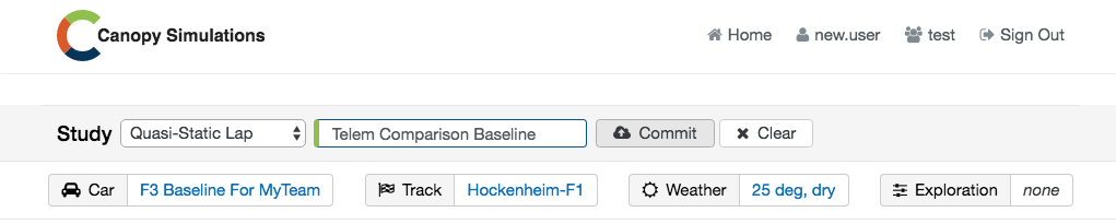
Step 1: Running a study with no Exploration defined yields a single baseline lap.
Step 2: Import your Telemetry
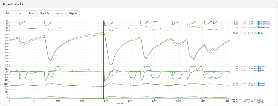
Viewing this study shows us the telemetry from our simulated lap. Above the chart we see a button marked Import which we click, select the data-file from our ‘real’ car and we are presented with an overlay of our simulated car telemetry and our actual telemetry:
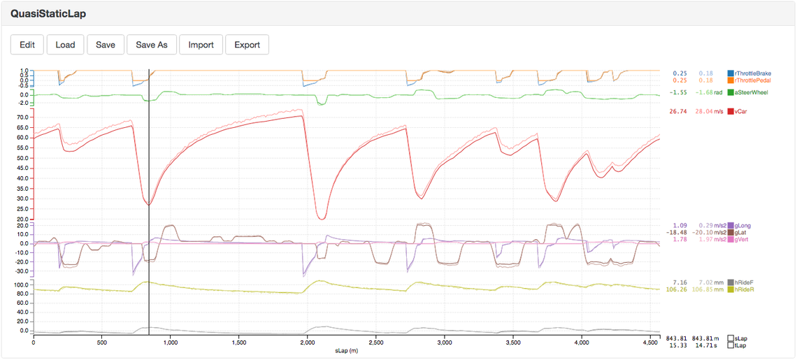
Step 2: Importing a telemetry file gives an overlay between simulations (dark) and telemetry (light).
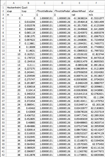
Step 2: The format for importing telemetry data is very simple.
The format for telemetry files to import is a simple .csv with a first line of metadata, a line of channel names, a line of units, and then many lines of channel values. You may need to create a custom chart to show channels from your telemetry files; this can be done easily in Canopy’s chart editor and saved as a custom chart for your team to use, and for you to further customise in future.
Note that the telemetry file which we have selected to import into the chart is not actually ‘uploaded’ to the internet, it’s just read and displayed by local code in your browser. As always with Canopy, the security of your data is paramount.
We can see from the chart above that our real car is faster than our simulated one on the straights and through the corners, both high speed and low speed, so we’ve got some tuning to do to get our parameters spot on for correlation with the track.
Step 3: Tune Overall Grip
This is where the power of the Canopy Platform really comes to the fore. Traditionally tuning parameters like grip, drag, and downforce to match model parameters to telemetry would be a painful process of editing and simulating, editing and simulating — relentless manual iteration through different parameter values. With the Canopy Platform we can sweep tens or hundreds of parameter values at the click of a button and not even tie-up our computer whilst doing it!
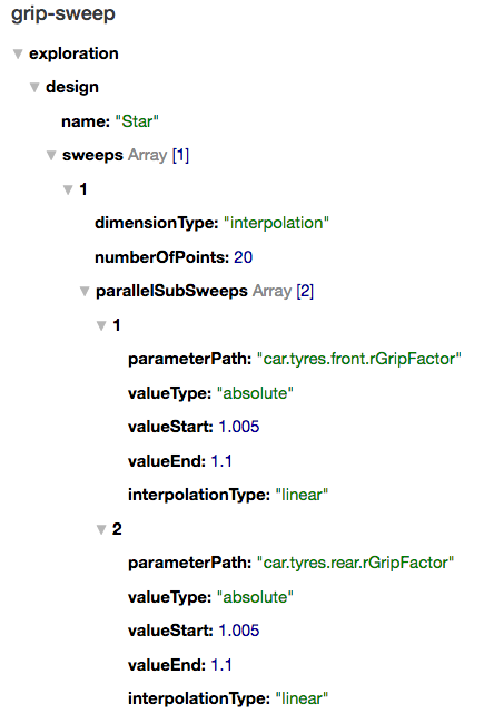
Step 3: A 20 lap sweep of front and rear tyre grip factor will help us to match low-speed corner apex speeds.
First of all, let’s sweep tyre grip factor until we match the speeds seen in telemetry at low-speed mid-corner. We can see that the baseline car is slower than telemetry in low-speed, mid corner, so let’s do a 20 lap sweep of front and rear rGripFactor from 1.005 to 1.1 and see whether one of those gets us close to the low-speed apex speeds of telemetry. Click on Exploration in the study staging area, New Exploration, name it, set the number of points to 20, then set the first parallel sub sweep of the first sweep definition to target the car.tyres.front.rGripFactor parameter and to sweep its value (value type absolute) from 1.005 to 1.1. Add another parallel sub sweep to the first sweep definition and set this one to do the same for the rear grip factor. When you’ve finished and clicked Create you should have an exploration which looks like the figure above left. Name this study and click Commit to once again leverage the power of the cloud against your parameterisation problems.
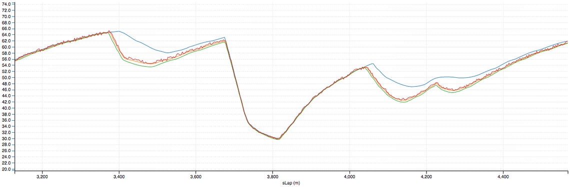
Once these 20 laps have been simulated we see straight away from the study view that the lap-time only approaches that of our telemetry lap (89.03s) towards the upper end of the grip sweep, so let’s throw the baseline lap, together with the 10th, 15th and 20th laps from the sweep into a chart and import our telemetry on top. Zooming in on the first apex we can see that somewhere between the 15th and 20th laps of the sweep seems to be in line with the telemetry:
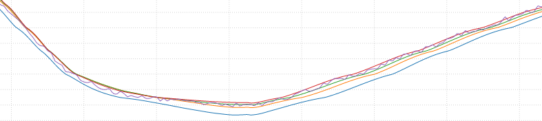
Step 3: Baseline (blue), 10th (yellow), 15th (green), and 20th (red) laps from the grip sweep plotted against the lap from telemetry (purple, wiggly) through the apex of turn one at Hockenheim.
The telemetry line seems to be above the green line more than it’s below it, so let’s choose a grip factor of 1.085 for the time being — we might revise this as and when we change the downforce level — meaning that lap 17 from our grip sweep becomes our new baseline.
Step 4: Tune Drag
The overlay between simulation and telemetry now looks like this, the laps being baseline (blue), 17th lap of grip sweep (orange), and telemetry (green, wobbly):
Step 4: The differences in EoS speed suggest that our baseline car is carrying too much drag.
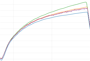
Step 4: The main straight for different drag levels; baseline (blue), -8pts (red), -10pts (yellow), -20pts (green), and telemetry (purple, wobbly).
The difference in end of straight (EoS) speed between the grip-corrected car and the telemetry is about 3m/s, or nearly 11kph. I don’t really have a good feel for how many points (100ths of a coefficient) of drag would make that kind of difference in EoS speed, so let’s just sweep between -1pt and -20pts of drag and see which looks closest to telemetry.
Again we create a new exploration, this time targeting the parameter car.aero. CDragBodyUserOffset with 20 drag values between -0.01 and -0.2. Before we commit this new study, we first must remember to update the staged car with our new grip levels; we do this by clicking on the staged car, then clicking Edit and changing the grip factor on both front and rear tyres to 1.085 before re-staging this edited car. Plotting the 10th and 20th laps from this sweep shows us that the right level is about the 8th lap of the sweep, adding this lap to the plot confirms our suspicions:
We again edit the staged car to cement this adjustment, either by changing CDragBodyUserOffset itself, or more likely by adjusting the coefficient of the constant term in the polynomial map for drag.
Step 5: Tune Downforce
So we have found a grip factor of 1.085, and a drag adjustment of -8pts; our vCar overlay between simulation and telemetry now looks like this:
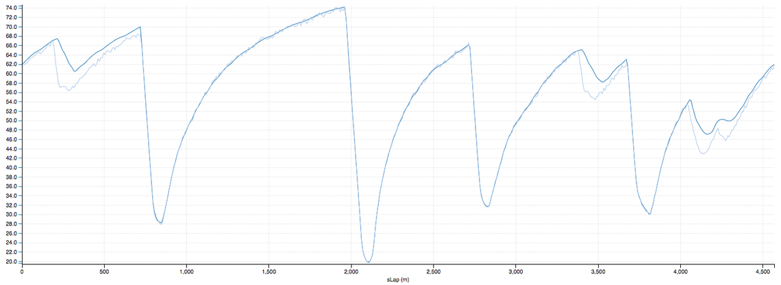
Step 5: After adjusting grip and drag we have this overlay between simulation (dark) and telemetry (light).
Clearly our simulated car has too much downforce, or more accurately our real car has too little downforce. This is a grimly familiar position for all of us who have toiled at the coalface of motorsport and battled the demons of the wind-tunnel. Let’s find out exactly what the ‘tunnel correction factor’ is in this case by running another 20-lap sweep, this time from -1pt to -20pts of CLT (Coefficient of Lift, Total). We can shortcut the creation of this sweep by starting from the drag sweep we just created; click New Exploration as before, but then select Staged from the import menu. Changing the name of the sweep, and the ‘Drag’ part of the parameter name to ‘Lift’ gives us the exploration which we desire. Click Create to finalise this exploration and then stage it with the up arrow button next to its entry in the explorations list.
Plotting the 1st, 10th and 20th lap from this sweep gives the following overlay with telemetry on final sector of the lap:
Step 5: The 1st (blue), 10th (yellow), and 20th (green) laps from the downforce sweep overlayed with telemetry (red).
The 10th lap is very close so let’s say that the CLT offset is -0.1, or in other words, the track seems to be 10pts down on the wind-tunnel.
Step 6: Bring it All Together
We once again edit the staged car to reflect this 10pt offset in CLT. Then we go to Cars, New Car, and this time import from Staged. This will create a copy of the staged car (which we’ve been editing with our new, tuned parameters). We name this one, save it, stage it and run a final single lap just to check our overlay with the finalised car:
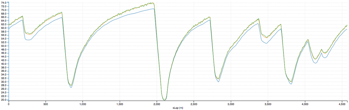
Step 6: Laps from our original baseline (blue), our new tuned car (yellow), and telemetry (green, wobbly).
It’s clear that our tuning of grip, drag, and downforce has brought the simulated lap into very close alignment with our telemetry lap. Our last change to the downforce offset will have slightly affected low-speed mid-corner speeds, which we brought into line with our initial tuning of grip, so we could go through each parameter again, re-using the explorations we’ve defined but with our new car as a baseline. For the purposes of this tutorial however, we’ll call it a day.
Bear in mind that we’ve concentrated only on gross car parameter adjustments, and on matching only the vCar channel from simulation with telemetry. In reality, there will be many more parameters to tune, and many more telemetry channels to compare to simulated ones. For instance, the many parameters of the tyre model can be tuned to match measured slip ratios, traction performance, braking performance, lateral loads, ride heights etc. etc. A great consolation in the face of all this complexity is that the Canopy Platform can run so many simulations, in such a short time, with such a high-fidelity vehicle model, that the full process of parameter estimation and tuning takes orders of magnitude less time than with traditional tools.
To recap: we’ve imported a telemetry file from the real car at Hockenheim and overlayed it with a simulation based on our parameterised car from part 2. We then swept through grip, drag, and downforce one after the other until we’d found the offset for each which best aligns simulation with telemetry. Now we’ve validated our parameterisation, we can do big setup or design explorations knowing that the results are well correlated to real car behaviour — meaning faster development, faster cars, and more silverware!
Keep an eye on our website or follow us on Twitter for future developments in this area — the upcoming addition of vector metamodels will further reduce the time taken to fit models to telemetry by changing the overlay live as you move sliders for each parameter.
To see how Canopy Simulations could help your team to move up the grid, contact us at hello@canopysimulations.com and arrange a live demo of the platform and talk to us about your team’s two-month free trial.