Getting Started 2: make it your car
AUGUST 9, 2016
In the first instalment of this series we went through signing-in to the platform and running a quick car mass sweep for Barcelona with the default car. In this second instalment we will create a new car with our own parameter data and run a more extensive exploration of its behaviour.
For this you will need:
Your sign-in details for the Canopy Platform (email us to arrange an online demo and start your evaluation period).
The parameters of your car, such as its mass, dimensions, engine map, aeromap, tyre parameters etc. etc. (don’t worry if you’re missing some information, we will cover that later).
We won’t go through all of the hundreds of parameters that are available to fully customise the Canopy car model to your particular car, but we will touch on each of the main groups of parameters, namely chassis, suspension, tyres, aero, brakes, control, and powertrain.
Step 1: Create a New Car
Picking up from where we left off in our previous article, click on the Car symbol in the study staging area (or go to Home>Cars), and then click the New Car button under the Car Configurations heading, this will bring up the new car editing/creation view:
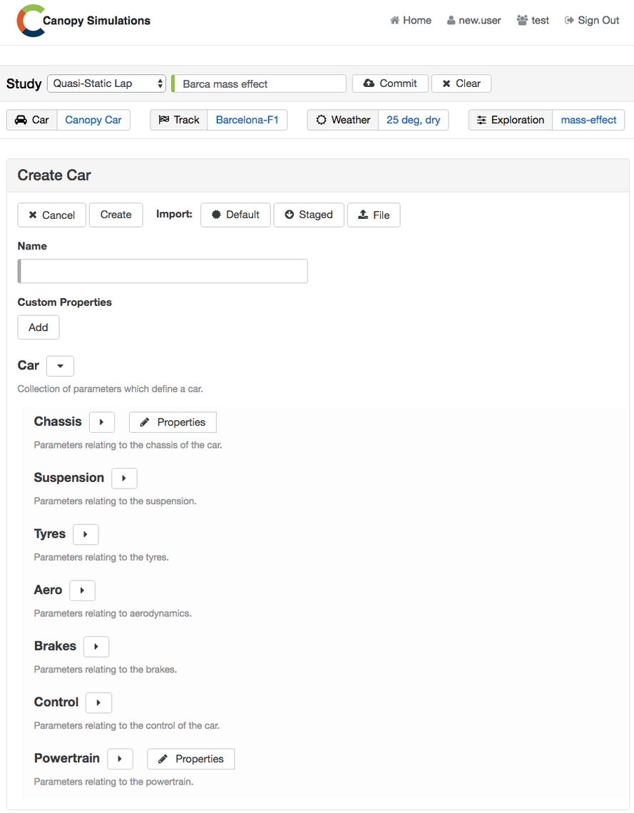
Step 1: Creating a new car with the built in parameter editor.
You’ll see that we are presented with options to import a car from several sources, Default, Staged, and File. These options will import all of the parameter data from either a default car, the car currently staged in the study staging area, or a car file which you have created offline, or more likely previously downloaded from the platform. In this case we’re going to import the default F3 car as an approximate starting place. Select Default from the list of import options, then select Canopy F3 Car from the list that appears below. Give your car a name, click Create, and you’ll see the car appear in your team’s virtual garage. Clicking on that car will bring up a view of the car’s parameter tree which you can explore to remind yourself of that car’s particular features. Clicking Edit will bring up the parameter editing view and we’re ready to start entering our parameters:
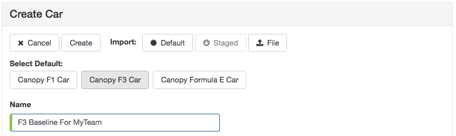
Step 1: By importing the default Canopy F3 Car we give ourselves a solid basis to customise with our own car’s parameters.
Step 2: Chassis
The car’s parameters are organised into a tree structure, the major branches are shown in the figure above. The first branch which we’ll explore is that relating to the chassis, or in some cases relating to the car’s overall mechanical properties. Expand the Chassis branch by clicking on the arrow and you’ll see the chassis parameters laid out ready for editing:
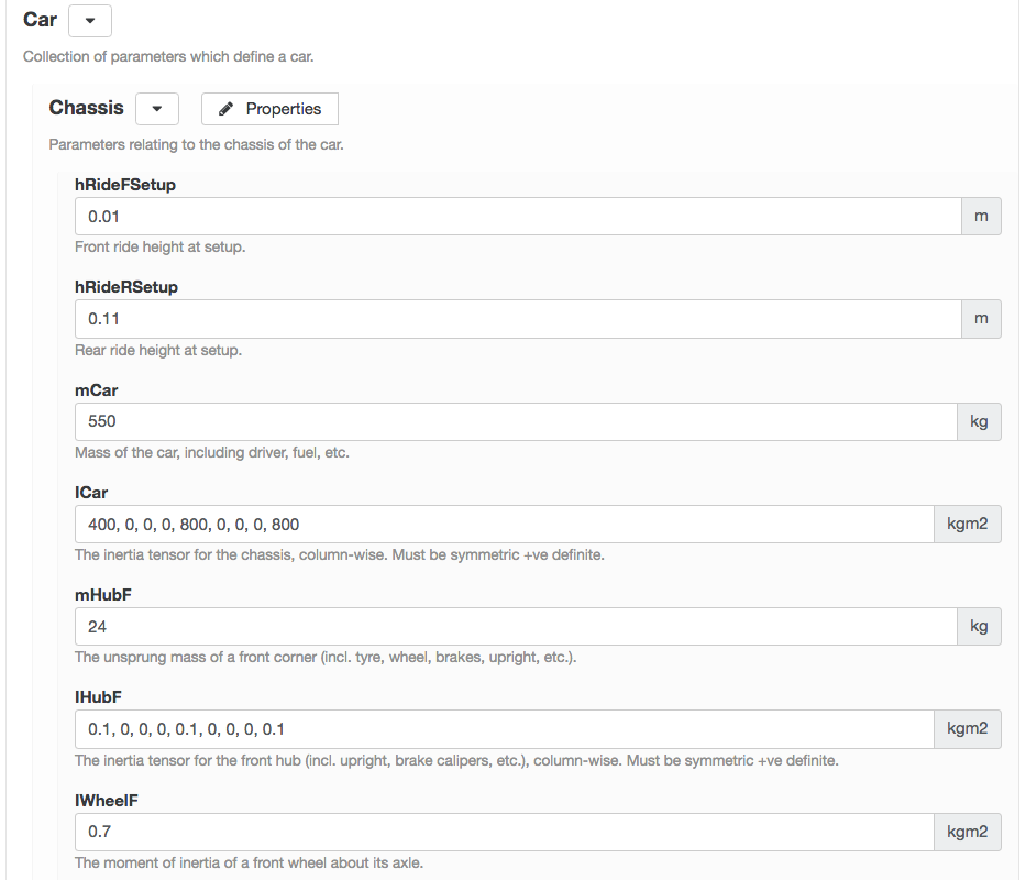
Step 2: The first few chassis parameters viewed in the editor.
The naming convention will be familiar to you already if you’ve ever looked at data from a McLaren ECU, otherwise here’s a quick introduction: the first letter denotes the physical type of the quantity (m=mass, h=height, I=inertia etc.) the second part denotes the thing that it relates to (Car, Hub, Wheel etc.), the third part denotes the position of that thing, if such a distinction is necessary (F=front, R=rear), finally we add any qualification relating to that channel and the condition it relates to, or the method of its measurement.
Here is where we can start entering the data relating to our particular car. The units of each number are shown on the right hand side of each edit box, and a brief description of each parameter’s meaning is given underneath. Fuller descriptions of the interpretation of the parameters are given in the aforementioned Canopy Wiki, with helpful diagrams such as this one:
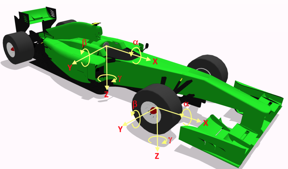
Step 2: Coordinate systems and sign conventions for parameters are explained in the Canopy Wiki.
It goes without saying that the more accurately you know the parameters of your car, the more useful the simulations will be for you. However, it’s also worth pointing out that you don’t need to know everything exactly to extract some very useful and applicable information from our simulations. We’ll see in the next installment that we can tune some key unknown parameter values by overlaying simulation data with real telemetry.
For the time being though, we enter all of the chassis parameters which we know, and have an informed guess at the ones we haven’t got numbers for, and then move on to the suspension.
Step 3: Suspension
Here we enter the spring, damper, and inerter characteristics as well as the pick-up-points for the front and rear suspension and the stiffness of a couple of elements such as the steering rack. Much like we entered the setup ride heights in the chassis branch, here we enter the setup camber and toe angles of the wheels:
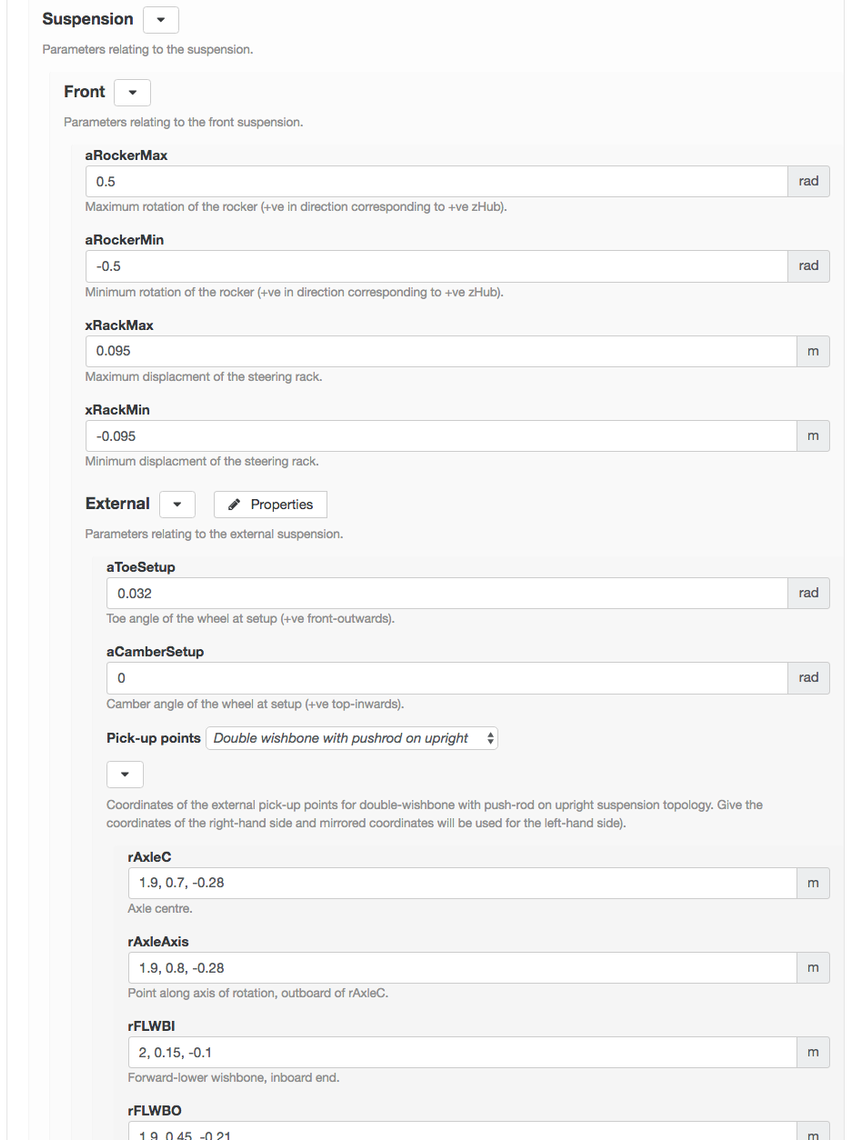
Step 3: Suspension parameters are comprehensive, including not only spring rates etc. but the pick-up points defining the suspension geometry.
The pick-up-points of the suspension are x-y-z coordinates of the pivot points of each part of the suspension (wishbones, track rods, etc.) both on the inboard (car) end and the outboard (wheel) end of each member. The Canopy model computes the kinematics of your suspension from these x-y-z coordinates each time a simulation is run, there is no need to use a separate kinematics package to transform pick-up-point locations into look-up tables, as is the case with many other simulation providers. Having said that, if you didn’t build your chassis yourself and you don’t have the coordinates of the pick-up-points, you can provide curves derived from a K&C rig instead of using the model’s internal kinematics engine.
As you can see from the previous screenshot (next to Pick-up points), you can choose when entering your pick-up-point values which topology relates to your car. In this case we’ve chosen Double wishbone with pushrod on upright but any suspension topology can be accommodated — if you can’t see yours already in the list, let us know and we’ll implement it for you.
Step 4: Tyres
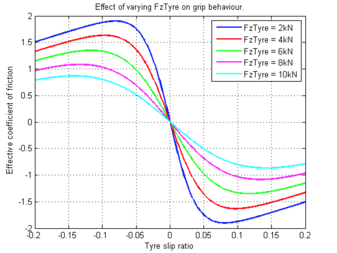
The Canopy car model doesn’t use the Pacejka formula, instead Canopy’s own tyre model is used, where all of the parameters have physical meanings. This makes it much easier to tune than the mysterious Pacejka model and it’s hundreds of nameless coefficients. If you have a set of Pacejka coefficients for your tyres we can provide a tool to convert them into an equivalent set of Canopy parameters which will give very similar force curves with a much more intuitive parameterisation. The Canopy tyre model is explained in detail in the Canopy Wiki and we are always on hand to help our clients to get the best out of it.
Sets of parameters representing certain tyre types or compounds (e.g., soft, super-soft, medium…) can be named and saved as components. This allows them to be easily re-used on different setups, or for the tyres to be easily changed on a particular setup. In fact this ability to save sets of parameters applies to all branches and all levels of the parameter tree, allowing you to build up your own library of named components and sub-assemblies for quick reaction to setup changes happening in your garage.
Step 5: Aero
Here we are, aero, the part of the parameterisation which is always guesswork, even if you’re an F1 team with two wind-tunnels and billions of flops of CFD. If you don’t have your own set of aerodymaniacs and you really don’t have a clue what your aeromap looks like, we recommend a visit to see a company such as TotalSim, who can CFD your car and give you an aeromap in no time. Once you’ve got some idea of how your car’s aero responds to car attitude (height, pitch, yaw, roll, steer) you can begin to parameterise the Canopy model.
The aeromap is represented as a polynomial surface in the Canopy model. Polynomial terms relating to the aerodynamic degrees of freedom are multiplied by coefficients and summed to give the overall lift and drag coefficients for any car attitude, this is most easily demonstrated with an example:
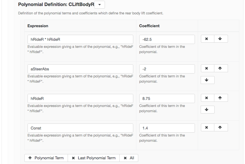
Step 5: The aero coefficient for rear downforce (CLiftBodyR) given by the sum of four polynomial terms, all of which are user-defined.
In the screenshot above we see that the rear downforce coefficient (CLiftBodyR) has been defined as:

This format of aeromap is very flexible and is able to accommodate many different aerodynamic effects in a very compact form. The aerodynamic degrees of freedom with which you can make your polynomial terms are: front and rear ride height, steering angle, roll angle, airflow curvature, yaw angles (overall, front, rear), front-wing flap angle, and a constant term. If you’re more familiar with aeromaps described by tables of lift coefficients over varying values of front and rear ride height, have no fear, you can upload your maps in that format and they will be dealt with internally.
The aero branch of the parameter tree also includes individual lift and drag coefficients for the front and rear wheels, as well as parameters characterising diffuser stall and of course user offsets for correlation and experimentation. If there is an important aero effect on your car which you can’t see reflected in the parameters, we can modify the model for you.
Step 6: Brakes
The brakes branch of the parameter tree is very simple, containing only three parameters for each axle:
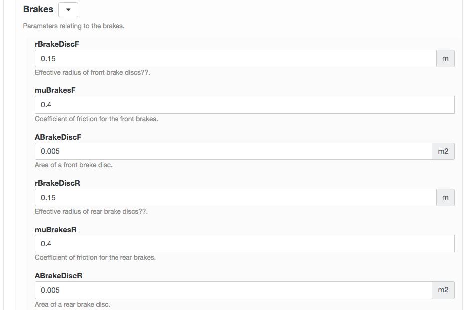
Step 6: The parameters of the brakes branch.
If brakes are of particular interest to your team, for instance if you’d like to simulate thermal effects such as heat-soak into the tyres, we can accommodate your needs.
Step 7: Control
The control branch contains only two parameters, brake balance and a stability limit which controls how much oversteer the simulation will allow:
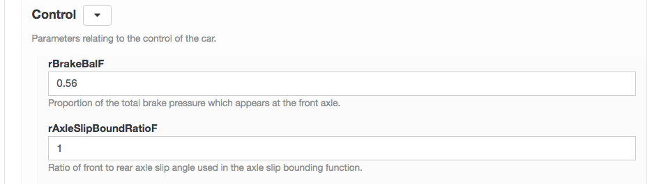
Step 7: Brake balance and stability limits are set in the control branch.
Step 8: Powertrain
Here’s where we copy and paste our engine map into the parameter tree and enter the details of our gearbox and final drive etc.
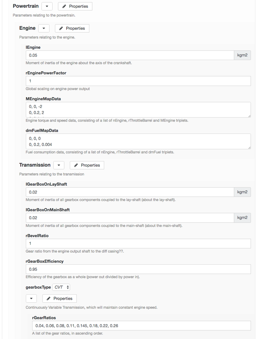
Step 8: The powertrain branch contains the engine maps, gear ratios, etc.
The format of the engine map data in the Canopy model is rows of three numbers, separated by commas, representing engine speed, throttle position, and engine torque. A few lines of Excel might be needed to get your engine map data into this format, again, we can supply templates for re-shaping if necessary. The same format is used for the fuel map. Although a set of tables might be more familiar, this format allows non-regular, non-gridded data to be entered — our model’s smooth interpolation function takes care of filling in between irregularly spaced data points, allowing you to specify the key regions of your map in arbitrarily high resolution without worrying about the unused portion of the space.
Both continuously variable transmission (CVT) and normal gearbox types are available in the Canopy model. Using CVT in simulation can be a useful way of preventing the results of broad-ranging studies from being polluted by ill-fitting gear ratios which have not been re-optimised for each setup.
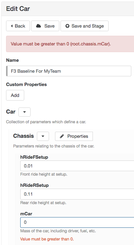
Step 9: Entering an invalid value (such as a zero car mass) will not go unnoticed for long!
Step 9: Miscellaneous
As you go through the parameter tree adding in your values, you’ll want to click Save every now and again to ensure that your work is not lost due to a shark biting through an undersea internet cable.
If at any point in the parameterisation process you accidentally enter an invalid value in one of the fields, you’ll see something like the screenshot shown to the left. Values are checked every time you move on to another box, so you can’t go far wrong without being alerted to the fact.
It’s worth noting at this point that the parameters you enter here are stored in your team’s dedicated secure database. They cannot be seen by anyone else, either from other teams of from within Canopy. Having spent a combined 26 years working for top F1 teams, we fully appreciate that your car parameters are secret and their security is paramount. You can rest assured that your parameters are completely secure on our platform and no-one outside of the designated group of team-members which you elected will be able to see them. You can manage access from within your team at any time, with nominated team administrators able to add and remove users themselves.
We’ve breezed quickly through all of the major branches of the parameter tree in this instalment and talked about how best to represent your car. In the next instalment of this Getting Started series, we will compare the simulation output from our newly parameterised car with some imported telemetry and fine-tune the tyre, and aero characteristics to bring the two into alignment.