Showing Our Sensitive Side
OCTOBER 2, 2018
There are some key facts about performance that almost every engineer in every F1 team should know. These are the “fundamental sensitivities” of the car. That is to say, if we change parameter “x” by a small amount, how much will that change lap time? A few key examples of this are as follows (all typical values for Barcelona):
Mass; the car will go slower by 0.03s per additional kg.
Downforce; the car will go faster by 0.03s per additional “point”.
Power; the car will go faster by 0.15s per % improvement in engine power.
Drag; the car will go slower by 0.06s per additional “point” of drag.
Centre-of-gravity height; the car will go 0.015s slower per lap for every 1mm rise in centre-of-gravity.
Every engineer should know these, because they form fundamental ready reckoners by which engineers can assess performance. If, for instance, a new engine is 0.5% more powerful (+0.075s), but weighs 1kg more (-0.03s) and brings up the CoG by 1mm (-0.015s), then it will yield about 0.03s. This is less than half the value of the pure gain in power. That’s worth having, but also well worth keeping a very close eye on the downsides; if the power delivery isn’t quite what you want, or the mass and CoG downsides are a bit bigger then all the benefit could disappear very quickly. Similarly, new performance concepts can be quickly assessed for whether they are likely to be worth pursuing — the famous F-duct was nearly scrapped because it added so much weight high up on the car.
The F-duct; it blazed a trail for DRS, but all that carbon high above the ground cost almost as much lap time as the aero benefits were worth in the first few iterations.
As useful as the “fundamentals” are for ready reckoning, they do not offer the kind of precision engineering for which F1 is famed. A single value of sensitivity for a lap doesn’t enable us to drill down and understand how or why the car will be faster or slower.
Local Sensitivities
In this article we are going to take a deeper look at the local lap time sensitivities. The picture below shows the a plot of the velocity of two cars going round turn 5 at Barcelona, then heading up the hill past turns 6 and 7. The cars are identical except that one of them has grippier tyres fitted. More grip means better cornering speed, but offers no benefit when we are limited by engine power rather than grip (actually there is a tiny benefit, but it’s close to zero).
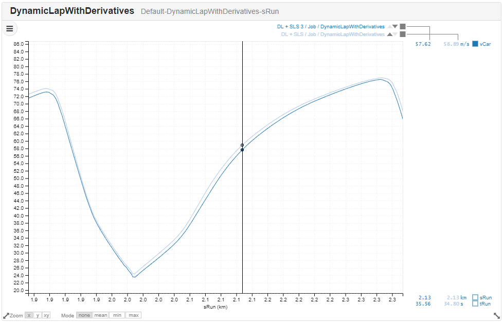
Turn 5, Barcelona for two cars which differ only in tyre grip. Despite the fact that all the lap time improvements are localised at mid-corner, the car with grippier tyres continues to gain all the way to the braking point.
Despite the fact that grip is only useful at mid-corner, we see that the car with grippier tyres continues to accrue lap time gains all the way to the braking point. This isn’t exactly rocket-science; if we go faster mid-corner then we can expect to maintain some benefit all the way along the straight. This is why we hear Martin Brundle and his co-commentators getting very excited about drivers “getting a good exit”; it means an overtake is possible, even when both cars have left the grip-limited part of the corner.
From an engineering perspective though, we don’t really want to see where lap time benefits accrue, we want to understand where they originate. On the Canopy Platform this question is answered in the form of Secondary Lap-time Sensitivities (or SLS). By the use of some nifty maths we can compute the sensitivity to any car parameter, localised to the points where the lap time benefits originate, rather than those where they are manifested. The picture below shows the Secondary Lap Time Sensitivities with respect to power.
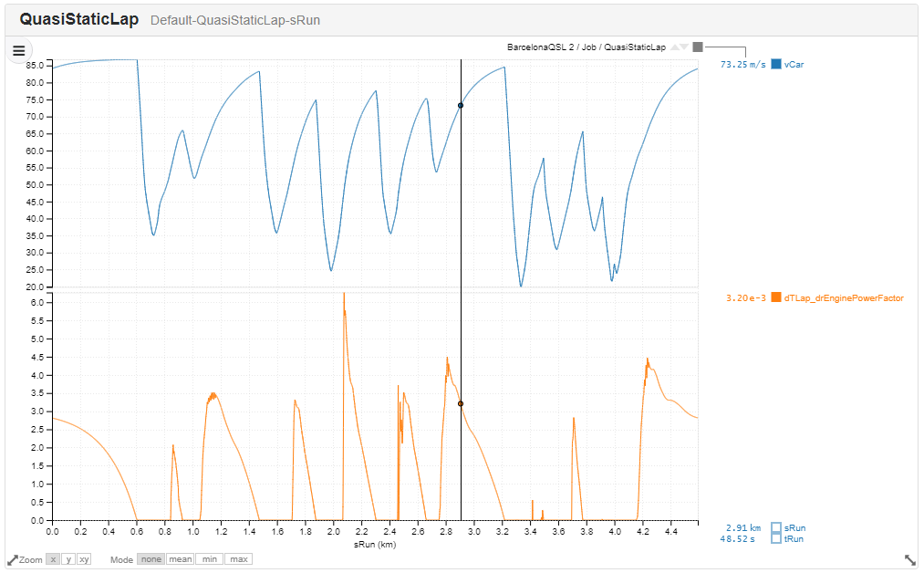
A lap of Barcelona, and the Secondary Lap Time Sensitivities for engine power.
This shows exactly the pattern we would expect. There is zero sensitivity at mid-corner, where the car is limited by grip. As we exit the corner sensitivity suddenly spikes, as the driver hits full throttle and the car becomes power limited. Lap time sensitivity to power diminishes as the car goes further along the straight, as the distance before the braking point reduces. We can play this game for all sorts of sensitivities; the figure below shows some of the SLS of the most interest.
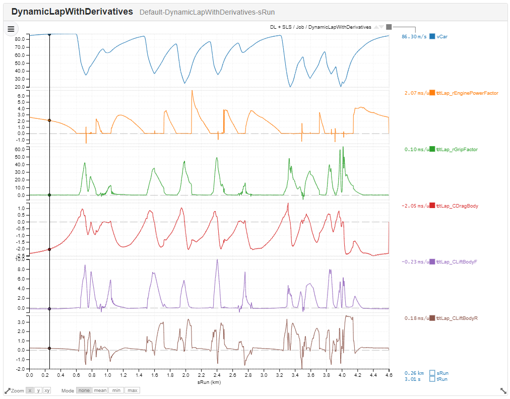
Secondary Lap Time Sensitivities for some of the biggest influences on car performance.
These are in themselves very interesting. For instance, although aero drag is generally a bad thing, under braking it’s actually helpful to performance. Similarly, adding rear downforce at mid-corner seems to be a performance detriment; this is likely because this car is very badly balanced and the solver has found the fastest way to get the car turned is to slide the rear. More downforce makes this harder to do. As soon as we can localise the lap time gains, we immediately see a much richer picture of exactly how common parameter changes will affect overall performance.
We can play some more advanced games with this technology. We can very easily extract the sensitivity to power, but plot it against engine speed. This graph could be waved under the noses of a powertrain supplier, telling them where more engine power will be most beneficial, across the operating range of the engine.
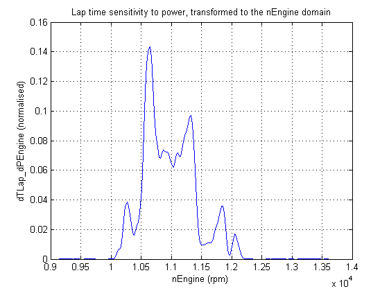
Lap-time sensitivity to engine power in the nEngine domain. One glance will tell a powertrain supplier to focus all their effort on the 10500–10750 rpm range.
A similar exercise can be played with aerodynamic performance, enabling aerodynamicists to target performance where it will count most. Applied in the right way, this is extremely powerful technology.
Quasi-Static Lap, our conventional Quasi-Static lap simulation has been churning these out for quite some time. A variety of clients have been extremely enthusiastic about this bit of technology; it’s gratifying when some of the world’s most respected racing teams feedback that a piece of technology has “changed our lives” or become “ubiquitous in the business”. The flipside to this enthusiasm has been consistent pressure for the SLS to be computed by Dynamic Lap as well. This has proved a huge technological challenge, which we are delighted to have finally cracked.
These cost a bit of execution time, but the results are lovely, and should entirely avoid some of the numerical issues that occasionally make life difficult for the Quasi-Static Lap version. In particular, we can see what happens when we look at the SLS for cars which are operating under energy or fuel consumption constraints.
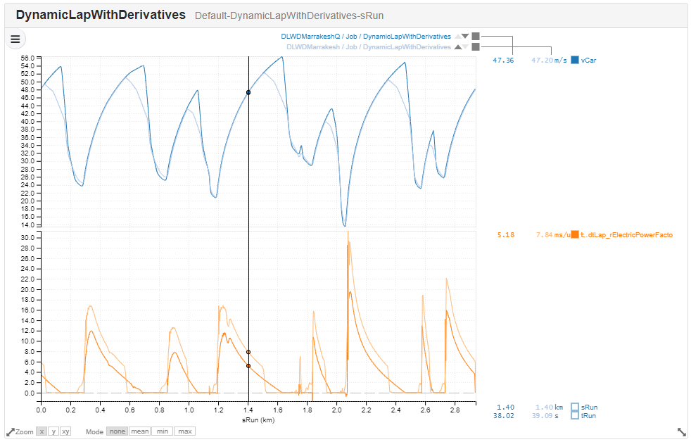
Two laps by the same Formula E car. In one case there is no energy constraint, as per Formula E qualifying. The other is more like a Formula E race, where energy is heavily constrained.
The figure above shows the power sensitivity for two Formula E cars going around the Marrakesh circuit. One of them has a severe energy constraint, while the other is doing something closer to a qualifying lap, with no energy constraint. As we can see the impact of a power boost in the power limited region is much larger for the car with an energy limit. This is for (at least) three reasons:
Because the driver is lifting off the throttle rather than accelerating all the way to the end of the straight, any speed gains will be maintained all the way through the coasting phase.
If you can get a Formula E car going faster, it means you can harvest more energy in regen and under braking. We still find it remarkable that the SLS channels are taking into account all the complexities of the powertrain energy flows and efficiencies.
Deploying a bit more power means deploying a bit more energy; the SLS channels are not taking account of the overall constraint on total energy used.
This leads us to a tricky question about how we handle the derivatives in the case where our resources are constrained. The mathematical interpretation of the SLS is “How much performance do I gain by changing a parameter at exactly this location?”. To answer the question about the performance we gain when changing power, on the other hand, we would have to ask “How much performance do I gain by changing a parameter at exactly this location, while optimally reducing power consumed at the most appropriate locations around the track?” Fortunately it turns out there is a simple rule we can follow.
If the parameter change directly causes an integral constraint to be violated, the aggregated lap time sensitivity won’t be accurate; this is the case where we change power factor in the presence of an energy constraint. However, if the parameter change doesn’t directly cause an integral constraint to be violated, the aggregated lap time sensitivity will be accurate; for example the case where we change aero drag in the presence of an energy constraint.
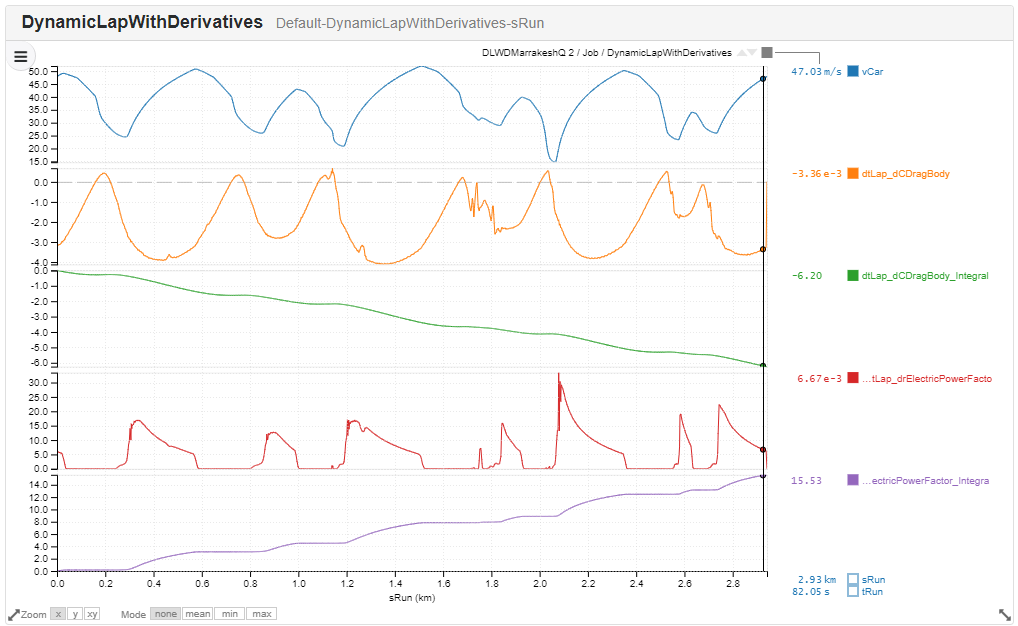
A lap of Marrakesh, and the sensitivities to power and drag. The power sensitivity suggests 0.15s per % electric power, but this is highly inaccurate as the addition of power requires the reoptimisation of the energy deployment. The drag sensitivity suggests -0.062s per point of drag. This is extremely accurate, despite the close relationship between aero drag and energy deployment strategy.
We’re looking forward to seeing what our clients make of this technology. All our client data is private, so we’ll never know if someone has developed a brilliant way of harnessing the power of SLS. We do know, however, that our clients are an imaginative bunch and we very much hope they exploit all the potential of this new technology.
If you would like to take a deeper look at what really drives the performance of your car, then please get in touch at hello@canopysimulations.com.