Race Preparation – Starting from Zero
JULY 14, 2016
These days simulation tools have a key role to play in almost all aspects of the operations of high-end racing teams. Throughout the life-cycle of a car, from concept design to race-weekend operations, the simulation tools used by the racing team will be being squeezed for all they are worth.
Nowhere, however, does a high quality set of simulation tools give such a competitive edge as when competing at a track you haven’t competed at before. Indeed in the case of Formula E, it might be that no-one has ever competed there before. Driver-In-The-Loop (DIL) simulators can be great tools for race-preparation, but with 1000’s of setup options to choose from, how do you even get started when all you have is a track outline supplied by the race organiser? You’ve got two options here:
Go back to the 1980’s, have a good stroke of your beard and make an educated guess.
Thrash your offline simulations tools for all they are worth.
Given our line of business, you won’t be surprised to hear we’re rather keen on option 2.
We’re going to illustrate this with the example of the fictional Madrid ePrix — as far as we are aware there is no Formula E race in Madrid, but a fictional track seems like a great place to start when discussing going to new tracks. Looking at Google Maps we think the following course might make a good basis for a track:
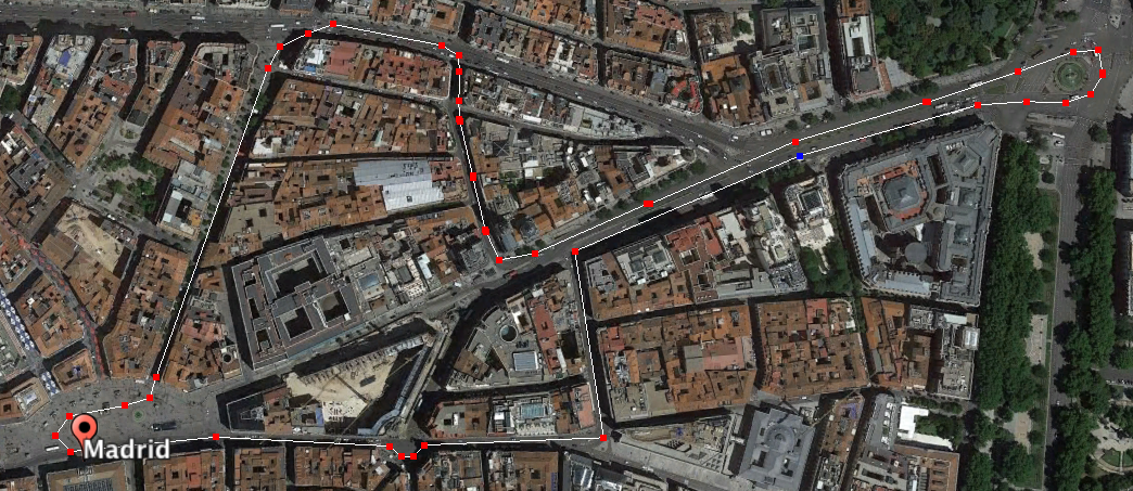
A good location for a Formula E race? Although we think one of the streets is pedestrianised, this looks pretty typical of the types of track Formula E visit. But when all you’ve got is a course outline, how do you prepare?
And at some point we’d hope that the race organisers would provide a track-outline. At this point we can start to get some serious value from our simulation tools. First off, we use the Canopy Simulations cloud platform to generate a racing line. At this point we start using phrases like “submit a track definition and car definition to the ‘Generate Racing Line’ tool” and it all starts to sound rather intimidating. However, we’ve made this extremely easy; I’ve just got the whole thing done in 11 mouse clicks. The resulting racing line easily passes the “looks about right” test. However, not only is that racing line ‘about right’, it’s actually exactly optimal, given the setup of the car we used for the racing-line generation simulation.
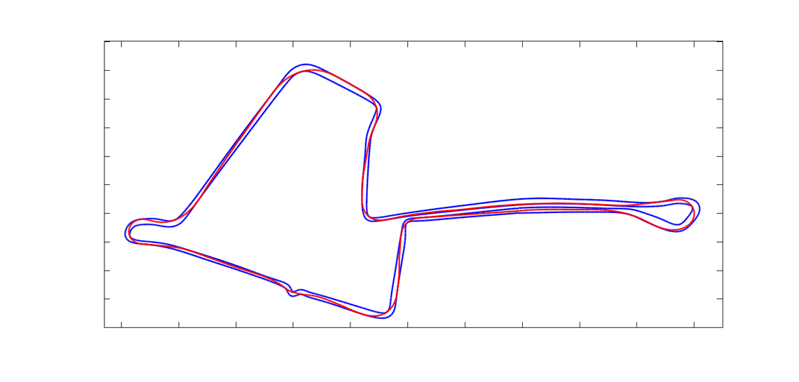
The Track outline and optimal racing line for the Madrid ePrix (in the event this race actually existed the organisers might want to tighten up the chicane).
Not only is the racing line optimal, but so is the deployment of electrical energy. We’ve allowed 6MJ per lap net energy deployment (although you can top this up by harvesting energy under braking). The figure below shows the best possible car velocity, energy deployment and energy harvest profiles.
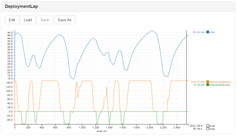
The optimal deployment profile for the Madrid ePrix. Note that there is insufficient electrical energy to complete the lap. The solver addresses this problem by coasting into each corner. Exactly how best to do this is a fiendishly hard problem, but the solution in the example above is exactly optimal.
The 6MJ per lap isn’t enough to go flat out down every straight, so our simulation has determined the best possible way of coasting towards each corner. Note that the car is also harvesting energy under braking and this allows further deployment beyond the 6MJ limit. Solving this deployment problem is a huge performance opportunity for Formula E, however, what we really want to know is not just how to make a given car go round a track as fast as possible, but how to make it go faster.
Once we can solve the simulation + deployment problem we can start homing in on the other areas of setup, in particular:
The fastest aerodynamic setup.
Best mechanical setup; springs, anti-roll bars, suspension geometries etc.
Formula E tracks tend to be tight and twisty, not unlike the Monaco F1 track. This immediately suggests high downforce aero configurations. High dowforce, however, tends to come with high drag and given the relatively low power of an FE car high drag should be avoided. Furthermore the limited electrical energy available should encourage the teams to run low drag configurations. Untangling the conflicting requirements of high downforce and low drag is virtually impossible without using simulation tools, and that’s where we can get a big leg-up from the Canopy Platform.
The car setup we used for the racing line and results shown so far is nothing more than a wild guess at what might be the best setup, so we probably have a great deal of ground to cover, and a great deal of potential to unlock. We are going to use the Canopy Platform to explore the entire setup space, and this will allow us to understand the performance landscape of the car. This is vital; without a rich understanding of the way car performance responds to setup changes, it is very difficult to combine the data generated by simulation with the human expertise and experience required to setup a car in such a way that the competing demands on the car, driver and race team are balanced. Furthermore, with a view of the whole performance landscape we can make sure we choose setups which are robust to changes in our assumptions.
Our experience (and also some maths) has shown us that somewhere in the vicinity of 1,000 simulations are required to explore the whole performance landscape. This is a large number, and a formidable challenge for most simulation packages. The challenges are two-fold; firstly how do you find the time and computing power to run 1,000 simulations, and secondly how do you extract value from such a large set of simulation results? Fortunately the Canopy Platform was developed from day one with this use case in mind. Designing the experiments we need is pretty trivial, and running the simulations even more so. Solving the optimal deployment problem is hard work, but it takes the Canopy Platform just 20 minutes to run all 1,000 simulations. This is transformationally fast by the standards of all other commercially available packages. It is also revolutionary in comparison to those packages which can’t solve the optimal deployment problem (we haven’t yet found another package which can solve this problem).
However, we are getting ahead of ourselves; what setup parameters do we want to change? In order to keep things relatively simple the following list seems like a good starting place:
Front and rear ride heights.
Front and rear spring stiffnesses.
Front and rear anti-roll bar stiffnesses.
Aerodynamic downforce coefficient in conjunction with the aerodynamic drag coefficient, capturing the fact that downforce and drag are inextricably linked.
We therefore have 7 ‘knobs’ that we can independently twiddle to make the car go faster. The effects of changing any of these parameters are cross-correlated with each of the other effects, so we need to explore the full 7-dimensional space to truly understand where to go with the setup. Note that although we have chosen these 7 setup parameters to explore users are free to explore the effects of absolutely any parameter associated with their car.
So here we are, approximately 20 minutes later, looking at the results of our performance scan. Firstly we can look at the parallel coordinates plot of the results to get a feel for the ‘shape’ of the performance landscape:
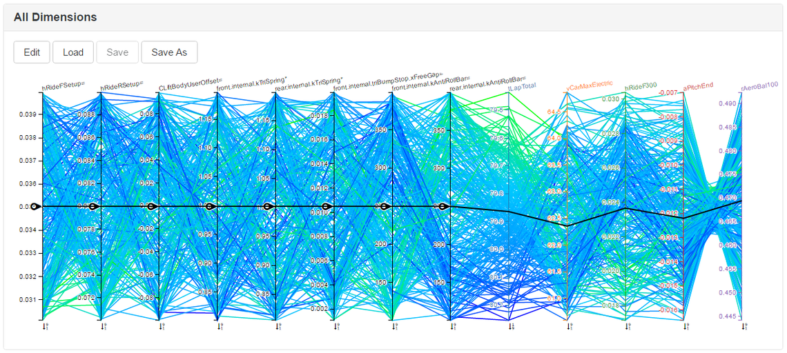
The parallel coordinates plot for the Madrid ePrix. Each line represents a single simulation. The leftmost 8 axes are the design variables, and the rest are the simulation results. The lines are coloured according to lap time, so clusters of light green suggest fast lap times, and clusters of blue slow lap times.
With a practised eye we can now pick out the areas of light green and immediately see that fast lap times seem to be correlated with:
Low front and rear ride heights.
Stiff rear anti-roll bars and soft front anti-roll bars.
Why this should be is something that your in-house performance miners will need to find out, but all the tools and data required to do so are available in the Canopy Platform.
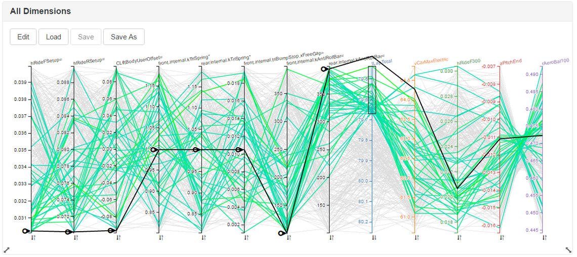
The same parallel coordinates plot as the previous one, but with the range of lap times restricted to those which are fast. The thick black line shows a candidate setup; the sliders on the left have been used to choose the design variables, while the rest of the line on the right shows the resulting outputs.
The parallel coordinates plot is great for getting a ‘feel’ for your car, but we can also look at slices through a response surface fitted to the simulation results. This gives a very clean look at how the various setup choices affect the response of the system.

Slices through a ‘response surface’ fitted to the simulation results. The sliders (circled in red) change the value of each design variable, as they do so, the graphs in the other three plots also change. In this case the sliders have been moved to what look like the best choices.
A text article is not the best place to demonstrate the power of the response surface viewer; it is by far best demonstrated in a video or live demonstration. However, by simply dragging a few sliders (circled in red in the picture) in the direction which looks like lap time will improve we can rapidly iterate our setup towards something faster. In this case for the price of 20 minutes of simulation we have got:
The optimal energy deployment profile for any setup we care to choose.
An improvement of about 0.7s on the performance of the baseline car, through mechanical setup alone.
Finally we can look at the aerodynamic behaviour:
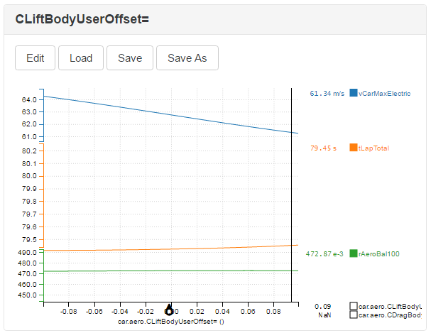
The response surface only for the aerodynamic sweep. Note that we assumed a 2:1 ratio of lift to drag; for every two units of downforce we also gained a unit of drag.
The graph is relatively flat with respect to lap time, although a low drag setup appears to be favoured. However, the strategic benefits of increased end-of-straight speeds mean that a low drag setup will almost certainly be the right choice. Before moving on we can compare the results of simulating this setup with the baseline car that we started with:
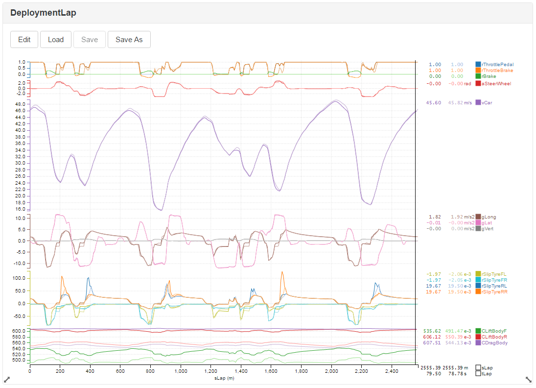
The overlay of the baseline car setup and the improved setup. The improved car can deploy further down the straights, offering a strategic advantage, and is also faster mid corner, due to the improved mechanical setup. All in all we’ve found 0.7s of performance — a good morning’s work!
We’ve had to guess most of the parameters for our example Formula E car, so we can’t claim that these results are directly applicable (not least because our track layout is fictional as well!). If, however, you happen to own your own formula E car and therefore know the car parameters accurately, then you could be very confident that the lap time discovered using these tools would manifest itself at the track.
It’s worth recapping what we’ve done here. In a little over half an hour we’ve gone from a bare track outline for a hypothetical Formula E ePrix, solved for the optimal power deployment and racing line on that track, then gone a long way down the road of finding the best mechanical and aero setup. Any team accessing this level of technology will immediately gain a big advantage on their rivals. Not only can teams use fundamentally more advanced simulations, but the rapid turn around times mean more design iterations and a deeper level of optimisation before and during a race weekend. Can any team afford not to exploit this technology?