Dynamic Simulation
MAY 2, 2017
We’ve been pretty quiet on the blogging front recently, primarily because life has been anything but quiet serving our platform clients. The clients themselves have also been pretty busy and we were really pleased to see the usage stats tick past 500,000 lap time simulations run since we agreed our first tenancy a year ago.
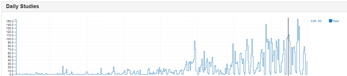
Daily studies on the platform since the first ever study we ran just over a year ago. Each study can consist of thousands of individual simulations: busy days have seen well over 10,000 lap simulations run on the platform.
Anyway, with a momentary easing of the manic pace, we thought we’d write about Dynamic Simulation and our latest simulation: DynamicLap, which think is well worth a bit of self-publicity. Dynamic lap time simulation is both the easiest and hardest from of simulation. In its easiest form dynamic simulation is of very limited value, but if you’ve solved the harder form then it’s among the most powerful tools any racing team can get their hands on.
Back in the early days of motor racing simulation some bright sparks thought, “if we can create a model of the car, we can feed it the same inputs as the real car, and find out everything we need to know before we get to the track”. That’s pretty much simulation in a nutshell, but the original simulations quite literally started a car rolling along the track, and attempted to drive it along. Without some pretty high quality control of the car you can’t do any very complex manoeuvres before stability becomes a major issue: go slightly too fast around slightly too tight a corner and you’ll spin out. So to solve this problem engineers started wrapping controllers around the car in order to do a better job of getting it around a corner in anything like a realistic fashion. The problem with this is that you can pay $30 million dollars for a decent car controller, and then just when it looks like it might be doing a decent job it heads off to drive the Indy 500. Replicating the skills of Fernando Alonso or his ilk is, to say the least, challenging. And even if you have a controller as good as a professional driver, you still won’t be able to resolve the fine detail that higher quality lap time simulation tools will offer. High level motorsport is all about stacking up benefits of a few hundredths of a second, and if your simulation tools don’t have the consistency to do this, it massively impacts their value.
The other issue with wrapping a controller around a car model and driving it round the track is you never know whether your car goes faster because it would actually go faster on a real track, or just because it happens to suit the characteristics of the controller.
However, dynamics are important, we can’t just wave away the need to handle them with an explanation about the fact that it is difficult. So what do you do if you want to implement a provably optimal dynamic simulation which handles:
Dynamics?
Racing line optimisation?
Track camber and gradient?
Limited quantities of fuel or electrical energy?
Environmental variations such as wind speed or track grip?
Resolution of lap time in fine grained detail?
The answer here it to use a mathematical technique known as collocation. Instead of starting with the car on the start/finish line and doing our best to drive it around the track we instead treat the entire lap in one go, and solve one big optimization problem. An optimization consists of two ingredients:
An objective function: the thing we want to be as small as possible.
A set of constraints: conditions we have to satisfy in order to have solved the problem.
In the case of lap time simulation, the objective is the lap time. The constraints should simply be that “the dynamics make sense”. This is seriously heavyweight stuff, so we’ll start with a really simple example and build up. The simple example is just a ball rolling down a hill: not very exciting, but subject to all the same physical laws as an F1 car.
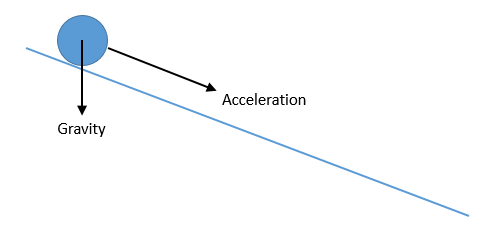
A ball rolling down a hill: it’s not exactly an F1 car zooming round Eau Rouge, but the laws of physics are the same!
A really simple way to solve the dynamics of this system is to split the ramp into, say, 100 elements then compute the acceleration of the ball at the start, integrate the acceleration to get the velocity at the next point. Repeat until you get to the end. This is pretty much exactly what the “naive” method of dynamic simulation does, except that instead of a ball, we have a car model.
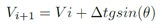
Velocity at the next time step is the velocity at the current time step plus acceleration due to gravity multiplied by the time step. This is a really bad way to do time marching simulation, but a really good way to explain Collocation.
We could change our perspective on this slightly and rearrange the equation above to give:
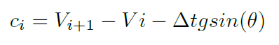
The previous equation, rearranged into the form of a constraint: if ci is zero then we’ve satisfied the system dynamics for the ith time step.
The dynamic equation has now become a constraint equation: if c is equal to zero, then we’ve satisfied the dynamics for that step. If every value of c is zero along the entire trajectory then we’ve satisfied the dynamics for the whole section (note that this is nothing like the way our collocation solver works, but it’s a nice way of explaining it). If, therefore, we solve the 100 simultaneous equations for the whole ramp then we manage to “simulate” a ball sliding down a ramp without ever solving the forward marching simulation problem. Now we’ve satisfied the constraints, what about the objective function? Well, we can change the problem from just solving the dynamics of a ball rolling down a ramp to finding out what shape of ramp will get the ball from one end of the ramp to the other as fast as possible.
Constructing this formulation takes a bit of thought, but we end up with an optimization problem with 305 unknowns and 248 constraints. Looking in from outside the world of optimization and high-kicking computational cleverness this seems pretty big, but it’s actually a very small problem. Optimizations start to get “big” when the number of unknowns goes past about 100,000, so only 300 is barely a warm up. The key point, here, however is that in just 0.2s we can solve this problem and generate the result of the famous “Brachistochrone” problem, first solved way back in 1697! (I think we can be pretty confident they didn’t do it numerically).
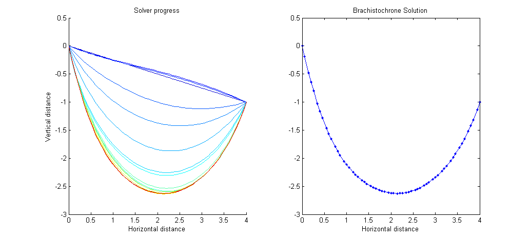
The progress of our optimizer solving the Brachistochrone. On the left hand side we start with a straight ramp, the colour then progresses through to red as the problem iterates towards the optimal solution. On the right hand side we show the optimal solution for the shape of a ramp down which to roll a ball in order to get to the other end as quickly as possible.
So this is pretty cool, we’ve solved the dynamics of the ball rolling down a hill, and also found out what shape the hill should be to do it as fast as possible. The question is: how far can we push this technology? The short answer is that if you use the numerical formulation I outlined above — not very far. However, with a huge amount of work and some specialist knowledge we can push it a very long way and start tackling some pretty complex systems: as complex as an F1 car going round a track or an America’s Cup yacht tacking upwind on its foils.
When solving the lap time simulation with an F1 car the track is split up into a large number of elements: about 1,000 “nodes” is a bare minimum for a short track like the Marrakesh Formula E circuit, while up to 10,000 nodes may be required for high resolution simulation of larger circuits. At each node there are about 50 different degrees of freedom and constraints, so we end up needing to solve a set of 50,000 non-linear equations. The picture below shows how the solver iterates its way to an optimal solution.
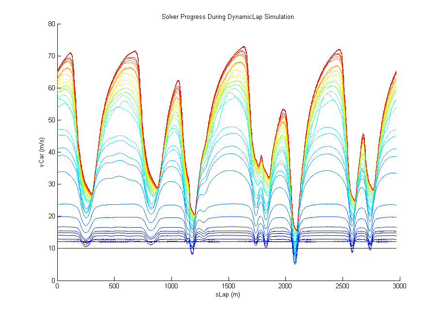
The progress of the optimisation solver for DynamicLap starting from a constant 10m/s until it has found the best possible solution. During the first few iterations not a great deal of progress is made, but then the solver makes rapid progress as the colours turn from blue to red. The last few iterations are spent nailing down the last few thousandths of a second.
All done in just two minutes! What we’ve actually done here is pretty remarkable (apologies for the total failure of modesty). We’ve optimized the racing line, handled all the dynamics of the car (it really is bouncing along the track) and optimally exploited a limited amount of electrical energy (although in this case there is enough electrical energy to go flat out everywhere). If we go back and change the amount of energy available the solver will reoptimize all the inputs, and minutely tweak the racing line to fit in with the new reality.
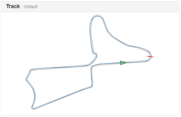
We’ve also optimised the racing line. Racing lines are a nightmare to visualise — the track is so narrow that viewing the whole track from above doesn’t show any detail. For a global view this is fine, but resolving fine details as the racing line changes is very hard.
With a few tweaks we can solve an even more complex problem: an all-electric car with an independent motor at all four corners. In this case, not only does retarding the inside wheel on corner exit get us out of the corner faster, it also enables us to save a bit of electrical energy. At this point my intuition begins to break down about what the optimal solution should look like; fortunately no such problems for DynamicLap:
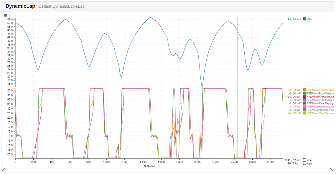
Results for a lap time simulation of Marrakesh with independently controlled 4-wheel drive. Every motor can do what it wants, when it wants, as long as it doesn’t exceed the energy allowance for the lap. Note that the optimizer is also exploiting the “regen paddle”: instead of coasting all the way to the end of each straight it starts harvesting before the braking point.
Readers with a passing familiarity with optimization problems such as these might start thinking “surely there are going to be loads of local minima for the solver to get stuck in: I can’t believe that consistency is going to be any good at all”. Well we’ve put in a huge amount of work on globalisation: ensuring that we find our way to a globally optimal solution. Show below is a plot of 100 simulations sweeping the rear ride height of a car in 0.3mm steps.
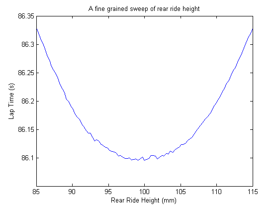
A fine grained sweep or rear ride height: while there is a bit of numerical noise note that the entire y-axis covers only 0.3s: the noise is of the order of thousandths. If your lap time simulation tools can’t generate this sort of graph, you won’t be getting all the value from them that you should.
There’s just enough numerical noise to be able to claim we haven’t made up the results, but this is the kind of consistency we’re looking for, that a lap time simulation tool which attempts to “drive” the car could never provide.
Other readers with a passing familiarity with optimization methods will look at these results and say “ah yes, but what simplifications have you had to make to the car model in order to get it to work?” — the answer to this is very simple: none at all. This is exactly the same vehicle model that we use for all our other simulations, and that we sell in compiled form for use in customers’ driver-in-the-loop simulators.
Here at Canopy Simulations we’ve been playing with this technology enough to come to the conclusion that it’s not just a useful way of solving a particularly tricky problem: this is the future of simulation. Yes it’s mathematically fiendish, and requires a certain amount of expertise to make it work, but the results are spectacular.
A natural question here is to ask where else this technology can be applied? Well the short answer to this is “anywhere we have a dynamic system that we want to control as well as possible”. A few examples that spring to mind:
An aircraft navigating a wind-field using the smallest possible amount of fuel.
A cargo vessel navigating a field of wind and tide using the smallest possible amount of fuel.
An America’s Cup yacht with constraints on human power output and course.
A road car going from A to B in a fixed time, using the minimum possible amount of energy; subject to upper and lower speed limits.
A robot attempting to optimize a manipulator path for speed, accuracy and efficiency.
This is just a short dip into the joys of how dynamic simulation “should” be done; we glossed over most of the details. However, if you are interested in exploiting this technology for your cars, or perhaps if you have a candidate problem you think we might be able to solve, do get in touch at hello@canopysimulations.com.