Introduction by Alex McCormick, Technical Director at Canopy

CANOPY in formula e

Formula E is a unique World Championship. Cars must complete each race using a finite amount of energy, balancing the need to get to the finish line first with the need to save energy, control tyre temperature, control battery temperature, and stay out of trouble on track.

To manage these complex and competing strategies, teams have made use of Canopy’s Dynamic Lap: our class-leading dynamic lap time simulation tool. Dynamic Lap is unique as the only commercially available vehicle simulation platform with the ability to provide guaranteed optimal energy strategies in the face of complex vehicle constraints – and it can simulate them all in virtually real-time.

Canopy has also been used to design and optimise some of the most unique developments in Formula E’s history. In such a resource and technology constrained environment, the smallest margins can be exploited for huge advantages.

Formula E: To lead, or to follow?

Unlike some racing series, the nature of the regulations and strategies in Formula E promote frequent overtaking and complex energy management strategies. Slipstreaming, or drafting, is used in other motorsports by a “following” car to reduce drag, ultimately gaining a speed advantage on the “lead” car which can translate into an overtake before the next corner.

However, in Formula E, drivers will make use of this drag reduction for another more subtle reason – to save energy. With the lead car punching a Formula E car sized hole in the air in front, the car behind can lift off earlier and coast for longer without losing ground – saving energy for a race-winning overtake later on.

The decision of whether to try to lead the race from the front, or to follow closely behind and to try to make an overtake late on in the race, is one that Canopy can help with.

Alexandra Gray’s MSc thesis attempts to quantify the possible savings by considering “slipstreaming” as an energy management technique instead of an overtaking aid. She considers the effects of the following car in a Formula E Gen 3 race.

AERODYNAMIC MODELLING

The study begins with a series of full-scale CFD simulations, characterising the aerodynamic behaviour of a simplified Gen 3 Formula E vehicle both in isolation and in the wake of a lead car, at separation distances of 0.5, 1.5, and 3 car lengths. 

The resulting aerodynamic coefficients are captured in the Canopy aero map, quantifying the lift and drag forces acting on the car at every vehicle state. A stall model was necessary to capture the aerodynamic behaviour at low rear ride heights.

The model was then validated against race telemetry by comparing push rod loads between track data and simulation results. To apply multi-vehicle wake effects, aerodynamic offsets were entered as coefficient adjustments in the car model.

Saving Up

“Push lap” simulations – used in qualifying, critical race phases, and energy-unconstrained scenarios – showed the expected physics: the following car gains a top speed advantage from reduced drag, but loses cornering and braking performance due to reduced downforce. The two effects largely cancel out over a full lap, with minimal net gain.

This is a common conclusion: “clear air”, or the absence of any car in front, is usually optimal for a one-off lap, because the downforce loss costs more time in corners than you can make up through the drag reduction in a straight line.

On “save laps”, where the driver must adhere to an energy target and therefore needs to lift and coast on the straights to save energy, the speed profile is very different.

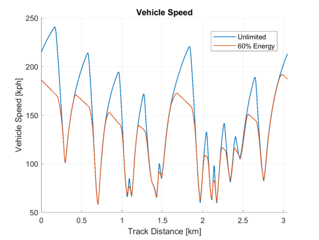
Thesis Figure 7: Push vs Energy Sector Vehicle Speed

It’s clear from this plot the “following” car could easily drive past the lead car just by deploying some extra energy – but they would pay for that later in the race. A far more interesting comparison is what happens when the “lead” and “follow” cars are both forced to drive to the energy target in a “save” lap.

cashing in

It turns out that the following car manages significantly higher top speeds, going a full 0.9s faster than the lead car while using exactly the same energy, even following at three car-lengths. The plot shows the speed overlay at a distance of 0.5 car-lengths, worth around 1.4 s/lap. 

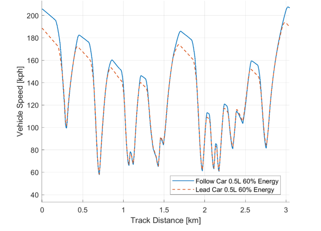
Figure 11: Vehicle Speed Lead vs Following Vehicle at 0.5L Energy Limited

That 0.9 s lap time makes it possible for the “following” car to stay in touch with the leader comfortably, leading to the queues of cars or “trains” so often seen in Formula E Gen 3 races. It allows the car behind more margin in the corners to manage tyre temperatures, more margin on the straights to manage battery and motor temperatures, and means mistakes don’t lead to losing touch entirely. 

Overtaking

At some point, in order to win a race, you have to lead it. The “following” car at some point needs to make a break for the line, and use its straight-line speed and energy advantage to make an overtake.

Alexandra’s thesis takes a novel approach to modelling overtaking – one that’s well worth reading the full article to understand. In summary, she demonstrates that when both the “lead” and “follow” cars are energy-constrained, the probability of an overtake is significantly increased.

conclusions

Formula E is a dramatic sport with dynamic, wheel-to-wheel racing and frequent overtaking – but it turns out the reasons behind this lie deep in the regulations and energy strategies chosen in the cars.

We can use Canopy’s Dynamic Lap to reveal some of the secrets behind high level motorsport, shining a light on the work done by the engineers and teams to overcome the technical and sporting challenges presented by the regulations and the strategy.

It is so much more than just a lap time simulator – its deep, fundamental design as a physics-based, engineering constrained optimisation tool allow engineers to explore questions like this one, understanding how to take advantage of a complex and counterintuitive system of regulations and strategy.

Many thanks to Alexandra for sharing a brilliantly researched and concisely summarised thesis with us! Read the full version here...

Canopy Simulation for Evaluation of Traffic Effects on Energy Management and Overtaking Opportunities in Formula E

by Alexandra Gray, MSc Researcher at Cranfield University

In a previous article, Rowland highlighted how secondary sensitivities in Canopy/Michelin’s lap time simulation,Dynamic Lap, are used to optimize driver inputs to meet a fuel savings target, leading to the well-established lift-and-coast technique. This article aims to illustrate how this functionality was adopted in a recent study to evaluate energy management strategies and overtaking opportunities for Formula E.

Series Background

In single make racing series such as Formula E, all vehicles have a common chassis and standardized aerodynamic packages. This allows a more direct comparison of driver ability and team strategy versus highlighting development differences in the vehicles themselves. 

One of the most influential factors in team strategy for Formula E is energy management as each race has a set limit on electrical power deployment. The current approach to energy management is to set sector targets for energy expenditure that minimize losses in lap time. In-wake aerodynamics present a possible alternative if the drag reductions associated with drafting, or following behind another vehicle, can be used as an energy management technique.

Study Background

Success in Formula E is dependent on an energy management strategy that minimizes losses in lap time and positions overtaken while operating in an energy sector. Taking inspiration from the fuel saving strategy of pack racing or drafting in NASCAR, an in-depth study was conducted to investigate in-wake aerodynamics as a potential method of saving energy.

Full scale computation fluid dynamics (CFD) studies were conducted to characterize the behavior of a simplified Gen 3 Formula E vehicle in isolation as well as in the wake of an upstream vehicle. Results of both studies were implemented into separate leading and following vehicle models for transient lap simulation.

This exercise was conducted for both a push lap and lap where energy was conserved using the lift and coast method. The results showed that exploiting the reduction of drag proved an efficient way to save energy through a sector that could then be deployed to overtake a competitor limited by an energy target.

Canopy Aerodynamic Model

The aerodynamic parameters for a vehicle in clean air was determined through a sweep of ride heights in CFD studies. Aerodynamic performance is recognized to be sensitive to yaw, steer, and roll, but changes in pitch for ground effect vehicles are the most influential; therefore, the aerodynamic performance was simplified to only dependencies on front (FRH) and rear (RRH) ride height for this study. For each simulation, aerodynamic coefficients were calculated for front lift, rear lift, and drag. Polynomials of varying order, such as the 2D quadratic equation for front lift coefficient (CLF) in Equation 1, were then fit to capture the behavior with respect to ride height and entered into Canopy as a base aero map.

Equation 1: Front Lift 2D Quadratic Equation

Canopy has the option to enter body and wheel loads separately. Polynomials are then added together to represent full vehicle behavior. For this study, all aerodynamic performance results from CFD were entered directly to the body definition shown in Figure 1.

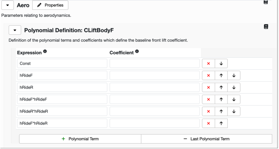
Figure 1: Aerodynamic Polynomial Definition

At first, rear lift coefficient as a function of ride height was fitted using the same form of 2D polynomial used for the front lift coefficient. While the quadratic polynomial was able to capture the general behavior, an additional offset was needed to capture stall behavior for the rear diffuser. Stall can be modeled as a rapid loss of downforce and drag between a ride height where the stall initiates (onset), and a second ride height where stall is complete as shown in Figure 2.

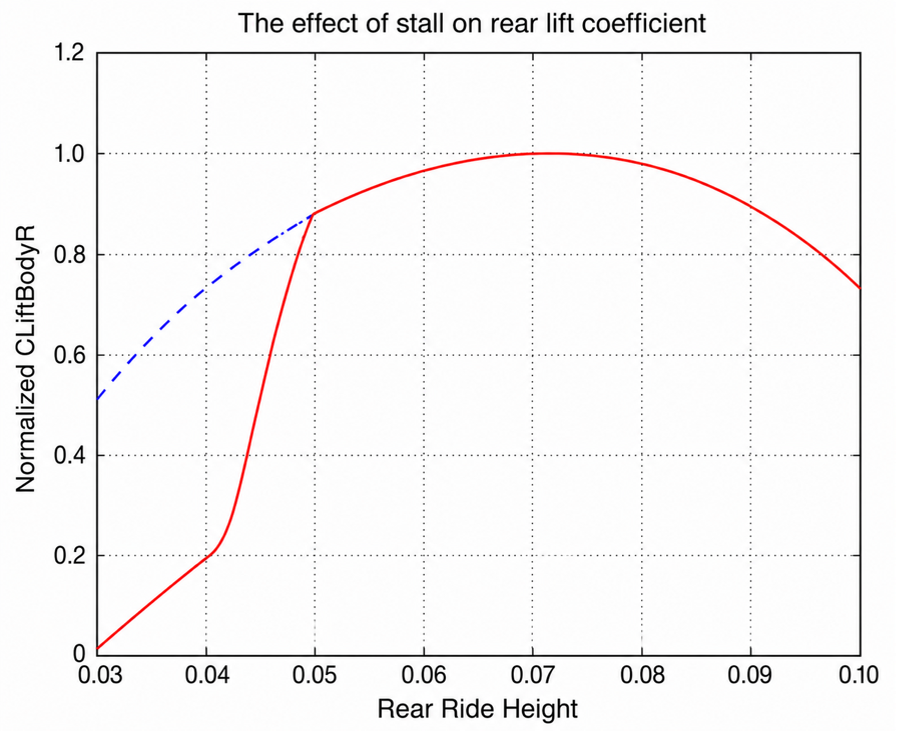
Figure 2: Effect of Stall on Rear Lift Coefficient

Canopy has two built in functions for aero stall: rear ride height and bi-linear. The rear ride height stall model fits a cubic spline between the stalled and unstalled points. It then defines a temporary stall ratio, t, which is linearly interpreted between the defined points. The stall ratio is used in Equation 3 to generate the fraction, r, by which the stall coefficient offsets entered by the user are applied.

Equation 2: Temporary Stall Ratio

Equation 3: Stall Fraction Rear Ride Height Model

For the bi-linear model, instead of defining a singular ride height, the user defines a line on the FRH-RRH map, beyond which the vehicle is completely stalled. The user must also input a second parallel line to the first one for the onset of stall. The temporary stall ratio, t, is now defined by the perpendicular distance between the current point and the completely stalled region. Similarly to the rear ride height model, t is used to define a temporary ratio, this time called rt, which is then used to define a final stall ratio using a continuous maximum and minimum limit as shown in Equation 13 and Equation 14.  Similarly to the first method, this ratio is then used to define the portion of the user defined offsets to apply. 

Equation 4: Temporary Stall Fraction

Equation 5: Stall Fraction Bilinear Model

For this study, the rear ride height method was used. The full aerodynamic model consisting of the base and stall polynomials was then validated against telemetry data by using a dynamic lap simulation and forcing the racing line to match that of the telemetry data. As downforce is a key contributor to vertical load along with weight transfer, the push rod loads were compared to telemetry to validate the CLF and CLR polynomials. The model followed both the rate of change of load and the median magnitude well across the track. Overall, the vehicle model captured the behavior of the car well. Differences could be attributed to wind effects in telemetry data as the simulation ran without an imposed wind condition, elevation, banking of the actual track whereas the canopy model was flat, and differences in driver input. None of these differences should not be a concern for the following analysis as all simulations were referenced against one another, not to the telemetry data.

Additional multi-vehicle simulations were then conducted at static ride heights chosen from a review of race telemetry as an average end of straight vehicle attitude. Separation distances of 0.5, 1.5, and 3 car lengths were chosen to capture behavior representative of just before an overtake, close racing, and regular running distance. As opposed to modifying inlet conditions for a single vehicle simulation, full vehicle simulations were selected so that effects could be captured both for the following vehicle due to the lead vehicle, and vice versa.

Offsets for aerodynamic coefficients at each following distance were calculated by comparing results to the isolated vehicle simulation at equivalent ride heights. These could be applied to any polynomial coefficient of each aerodynamic coefficient expression. Offsets were applied to the aero section of the car model using the user coefficient offsets which then became active for the entirety of a lap.

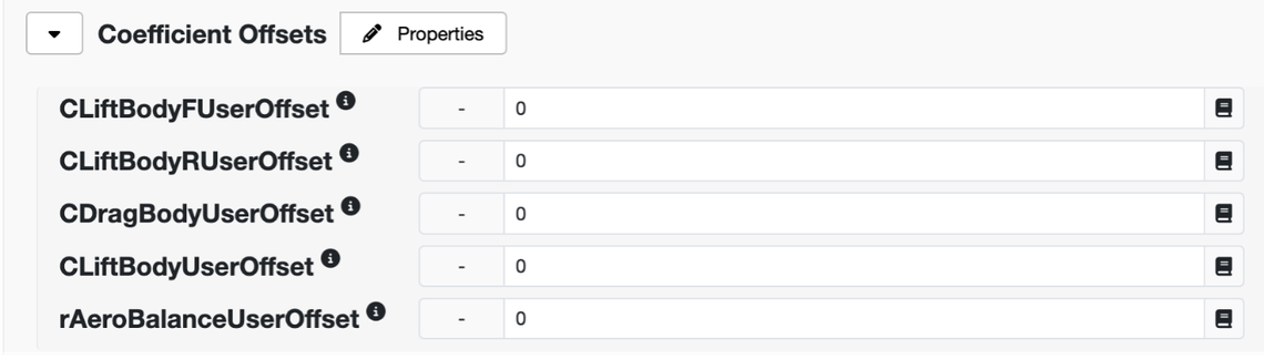
Figure 3: Offsets for Full Lap Traffic

Canopy Powertrain Model

The other key feature for this study was the ability to regulate the maximum allowable net energy deployment per stint/lap by modifying the EDeploymentRegulatoryMax parameter under the storage options for the electric motor. In Formula E, the FIA sets a defined amount of energy allowed per race which is typically around 25 percent less than the required amount to complete the race at full power for all laps. This practice forces teams to implement energy management strategies such as energy sectors where drivers are limited not by the performance of the vehicle, but by a maximum allowed energy expenditure. Target lap times are then decided by using an energy frontier which allows strategy engineers to identify an energy target per lap (in kWh) with the least possible lap time penalty. For the sake of modeling, a target value of 60% of the push lap for an energy saving lap or sector was used.

To conserve energy while maintaining a competitive speed, the most common approach is a lift and coast technique where the driver reduces input to the throttle and allows the vehicle to coast by its own momentum or with some amount of regenerative coasting torque. Figure 7 shows a comparison of the speed profiles of two dynamic lap simulations, the vehicle on a push lap with unlimited energy versus a 60% energy target, where this lift and coast behavior is captured. 

Figure 7: Push vs Energy Sector Vehicle Speed

Canopy Dynamic Lap Simulation

Dynamic lap simulations achieve the maximum performance of the car without assumptions from a driver model. The simulation solves every state of the car model at each point on a specified track racing line. Important for Formula E, the simulation allows users to impose energy/thermal constraints and control inputs for brake balance. Results can easily be exported for further analysis, such as to Matlab for this study.

In this study, the dynamic lap simulation was used to evaluate the impacts of aerodynamic wake behavior. As this simulation is built for a single car, multi-vehicle effects were entered as offsets and modifications made to the vehicle model, then the simulation data of a lead and following vehicle setup were compared to one another directly. To force this following behavior, the race line was defined in Canopy instead of allowing the race line to be optimized within the track limits for each setup.

Lap simulations were run for two conditions: push laps and energy saving laps. Push lap simulations assumed that both vehicles are at equal power, running the same race strategy for energy conservation, and therefore the recorded gaps are the sole result of aerodynamic wake effects on the vehicle. Separate simulations were run at each of the longitudinal separation distances. For each condition, simulations were run to assess the impact of running an entire lap in traffic, versus running in traffic through defined potential overtaking sectors.

Full Lap – Push

Initial simulations applied the longitudinal separation losses across an entire lap. A G-G diagram such as Figure 8 considers the lateral and longitudinal accelerations of the vehicle and can be used to characterize the performance of the driver-vehicle system. Ideally, the circle should be expanded outwards as much as possible. The relatively flat top of the diagram shows the vehicle is limited by the maximum power deployment’s ability to overcome drag and rolling resistance. Although the following car has significantly less drag, the greater forward longitudinal acceleration of the lead car suggests that the following car is traction limited. This aligns with the fact that the following car is also generating less downforce than the leading car. The additional downforce of the leading car allows for higher braking accelerations and lateral accelerations. Looking at Figure 9, this greater lateral acceleration due to downforce explains why the lead car is faster than the following car through the corners.

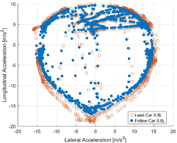
Figure 8: G-G Diagram for Lead vs Following Vehicle at 0.5L

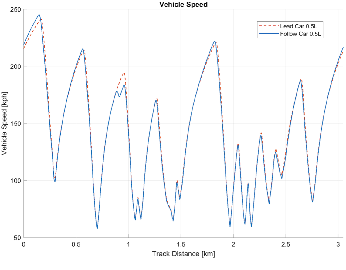
Figure 9: Vehicle Speed Lead vs Following Vehicle at 0.5L

Comparing the change in electrical energy deployment between the leading and following vehicles for each following distance, Figure 10 shows that close following distances allow the following car to save on electrical deployment. This explains why Formula E vehicles spend time pack racing or in the slipstream of another vehicle saving up energy so that it can be deployed to create a power difference when attempting an overtake.

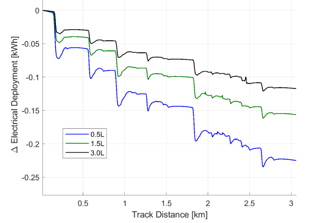
Figure 10: Change in Electrical Deployment from Lead Car with Separation

Full Lap – Energy Saving

Looking instead at a full lap where both the lead and following car are on an energy saving strategy, Figure 11 shows the following vehicle can maintain almost the same minimum speeds as the leading vehicle. CFD offsets for this vehicle showed the coefficient of lift for the leading vehicle is more negative, generating more vertical load which increases the braking force and resulting braking torque. To achieve the same braking torque, the following car must brake longer and harder as shown in Figure 12. 

Figure 11: Vehicle Speed Lead vs Following Vehicle at 0.5L Energy Limited

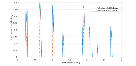
Figure 12: Braking Input Lead vs Following Vehicle at 0.5L Energy Limited

At the same time, due to the loss of drag, the following vehicle can deploy equal or less electrical power as shown in Figure 13 and still have a higher top speed than the leading vehicle on almost straight and corner exit. Over the course of a lap this results in a 1.375 second faster time at a following distance of 0.5 car length using the same total electrical power.

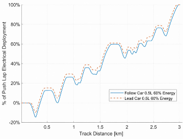
Figure 13: Electrical Deployment Lead vs Following Vehicle at 0.5L Energy Limited

This trend holds for all following distances although the effect decreases as distance increases as shown in Figure 14 and Figure 15. The respective reduction in lap times for the following car across the full lap for 1.5 car lengths and 3.0 car lengths are 1.0816 and 0.9086 seconds. 

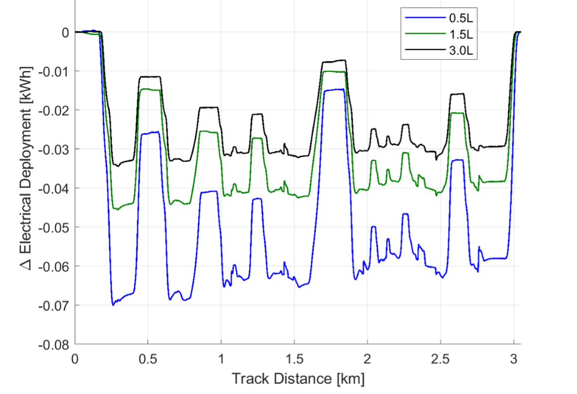
Figure 14: Change in Electrical Deployment from Lead Car with Energy Limitation

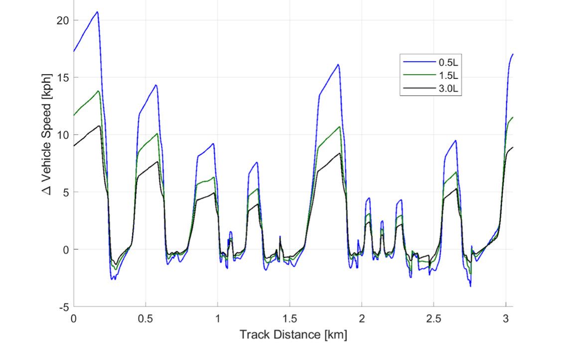
Figure 15: Change in Vehicle Speed from Lead Car with Energy Limitation

Overtaking Sectors

Potential overtaking sectors were determined based on the regions of the track where the following car vehicle speed was 5 kph or greater than the leading car for all three longitudinal separation distances. As this did not occur in the push full lap analysis, push laps were evaluated in segments where vehicle speed was 1 kph or greater than the leading car for all three longitudinal separation distances. Additional margin was added to capture entire track features instead of ending or starting mid-corner.

Table 1: Energy Limited Potential Overtaking Zones

A simplified approach to overtaking is that a successful overtake is dependent on the time gained in a sector compared to a leading car. An overtaking probability (Po) function was generated using historical Formula E race data where tgain is the time gained per sector. Gain is calculated from the perspective of the trailing/overtaking car as the difference between the end of sector time gap and the sector start time gap between two vehicles. The sign convention for gap is defined as positive for being behind a leading car and negative for being in front of an overtaken car. Using this sign convention, negative gain indicates that the gap between the trailing and leading car has increased and an overtake is not possible.

Sectors 1, 2, and 5 correspond to the three sectors evaluated for the push lap. Table 2 shows that the energy limitation creates the most probable overtaking scenarios in sector 1 followed by sector 5 for all separation distances. These zones are characterized as being two of the three highest speed sections of the track, suggesting that the influence of wake aerodynamics is greatest at high speeds. However, the top vehicle speed in sector 2 (S2) of 182.3 kph is within just under 2% of the top speed of sector 5 (S5) at 185.9 kph, yet the maximum overtaking probability is only 10.8% compared to 17.1%. Both sectors are straights, and in both cases the same following distances are evaluated, so the limits of vehicle performance are equal.  The difference between the two sectors is total length: 0.18 km for S2 and 0.23 km for S5. Carrying the same aerodynamic advantages compared to the lead car for the entire sector, this results in cumulative energy deployment savings of 41.3 W for S2 and 49.5 W for S5. This energy can then be deployed for overtaking resulting in a greater change in speed from the leading car (14.3 kph for S2 and 16.1 kph for S5). 

This reinforces the finding from full lap analysis that spending additional time at close length behind a leading car increases the potential energy savings which increases overtaking probability. 

Table 2: Overtaking Probability for Energy Limited Longitudinal Separation

As shown in Table 3, the percentage difference between following at 0.5L vs 1.5L in sector 1 increases from 23.8% to 51.8% for push versus energy sectors. This shows the influence of following distance on wake aerodynamics is far greater when coupled with additional factors, such as energy management, that generate a speed differential. 

Table 3: Overtaking Probability Push vs Energy Sector

Conclusions

In summary, this study showed the importance of including inter-vehicle wake influences when using transient lap simulations as wake aerodynamics significantly alter the capabilities of a vehicle’s performance. While simple, the implemented overtaking model allowed for direct evaluation of overtaking success probability. When combined with the effects of energy conservation, harnessing wake aerodynamics proved an efficient way to exploit existing speed differentials and increase the time gained per sector over a competitor.

The above study shows just one example of how existing functions in Canopy can be repurposed to fit the needs of specific investigations. While this study made many simplifications, the process for modeling aerodynamic vehicle behavior, enforcing energy constraints, and evaluating energy deployment and the influence on overtaking opportunities can be carried forward into other series and at higher levels of accuracy.

This approach investigated a single longitudinal offset, applied instantaneously and maintained throughout either the entire track or through a defined sector. Similarly to how temporary ratios are used in the aeroStall function to vary the stall offset for different ride heights, a function should be defined to distribute a portion of the following or leading offsets dependent on the distance to the defined sector. Literature review also highlights the influence of side force throughout the overtaking maneuver on top of offsets to lift and drag, which could be easily implemented after additional CFD studies using the same methodology.

Alexandra Gray - Linkedin.